import ibis
from ibis import _
ibis.options.interactive = True
import pandas as pd
from plotnine import ggplot, geom_line, aes


household = ibis.read_parquet("pums_household/*.parquet",
hive_partitioning=True)Part 3 – Data Wrangling with Ibis
Learning objectives
- Explain the value of Ibis for data analysis
- Write data queries using Ibis to get insight from data
- Apply chaining to combine operations
Introduction to Ibis
In this part of the training, we want to do some analytics work to get insights from the data. To do this we will be using Ibis.
Ibis is a Python library that provides a lightweight, universal interface for data wrangling. It helps Python users explore and transform data of any size, stored anywhere.
To do this, under the hood Ibis compiles and generates SQL for many backends, including MySQL, PostgresSQL, DuckDB, PySpark, and BigQuery, amongst others. Ibis currently supports 15 backends and counting!
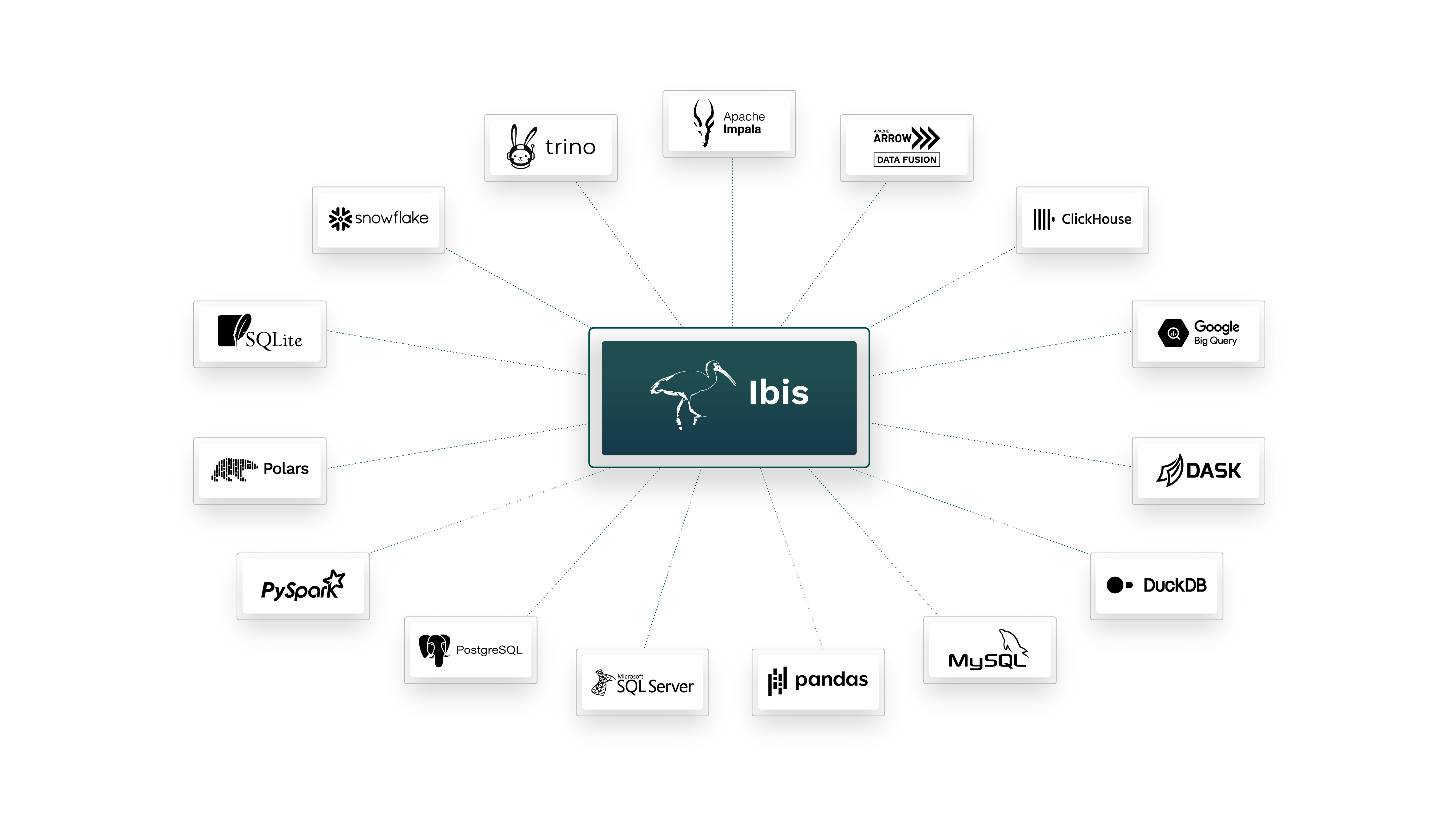
Additionally, with Ibis, the code used for queries is independent from the backend. If the data are moved to a different system (PostgreSQL, SQLite, Google BigQuery, etc…), the code will not need to be rewritten.
Ibis has excellent read_csv and read_parquet functions that can let you access and analyze data quickly! These methods use the DuckDB engine as their default and will be what we’ll start with today.
Later you will work with data stored remotely in Snowkflake to see how to switch between backends.
Analysing the Data
Let’s now use Ibis to wrangle and analyse our data. We’ll start by importing the dependencies we need and reading in the parquet files for the household data.
household is now an Ibis table that you can query in a similar way that you would a pandas dataframe. PUMS contains a very long list of columns and the column names are not very intuitive. You can find the full list of columns, they’re names and the data they contain here.
Owner and Renter Occupied Housing by Age
For this first part of the tutorial we will specifically be using the TEN and HHLDRAGEP columns to create a graph that shows owner and renter occupied housing by age.
Here are the questions asked to get the data for these columns:
TEN Character 1
Tenure
b. N/A (GQ/vacant)
1. Owned with mortgage or loan (include home equity loans)
2. Owned free and clear
3. Rented
4. Occupied without payment of rent
HHLDRAGEP Numeric 2
Age of the householder
bb. N/A (GQ/vacant)
15..99. 15 to 99 years (Top-coded)We’ll start by grabbing the necessary columns, filtering out nulls and relabeling the columns names. Here’s the code to do this:
tenure_type = (
    household
    .select('HHLDRAGEP', 'TEN')
    .filter(_.TEN.notnull())
    .relabel(dict(
        HHLDRAGEP="age_householder",
        TEN="tenure_type",
    ))
)
Note
Run this and print head of this table
Next we’ll use mutate to add two new columns tenure_type and age_group to the table. These will be used to:
- recode the different types of home ownership, and;
- bin the householder ages into groups.
This operation will allow us to have clearer categories when using the group_by function to calculate the number of people in each group.
tenure_type_age_group = (
    tenure_type
    .mutate(
        tenure_type=ibis.case()
        .when(tenure_type.tenure_type == 1, "owned_with_mortgage")
        .when(tenure_type.tenure_type == 2, "owned_free_and_clear")
        .when(tenure_type.tenure_type == 3, "rented")
        .when(tenure_type.tenure_type == 4, "no_rent")
        .else_("missing")
        .end(),
        age_group=ibis.case()
        .when(tenure_type.age_householder < 25, "Under 25 years")
        .when((tenure_type.age_householder >= 25) & (tenure_type.age_householder <= 29), "25 - 29")
        .when((tenure_type.age_householder >= 30) & (tenure_type.age_householder <= 34), "30 - 34")
        .when((tenure_type.age_householder >= 35) & (tenure_type.age_householder <= 44), "35 - 44")
        .when((tenure_type.age_householder >= 45) & (tenure_type.age_householder <= 54), "45 - 54")
        .when((tenure_type.age_householder >= 55) & (tenure_type.age_householder <= 64), "55 - 64")
        .when((tenure_type.age_householder >= 65) & (tenure_type.age_householder <= 74), "65 - 74")
        .when(tenure_type.age_householder >= 75, "75 years and older")
        .end()
    )
    .group_by([_.age_group, _.tenure_type])
    .count()
)
Finally we’ll use plotnine (the Python version of ggplot) to render the graph:
pdttag = tenure_type_age_group.to_pyarrow().to_pandas()
pdttag['age_group'] = pd.Categorical(pdttag['age_group'], ordered=True,
                                     categories=['Under 25 years', '25 - 29', '30 - 34', '35 - 44',
                                                 '45 - 54', '55 - 64', '65 - 74', '75 years and older'])

a = (ggplot(pdttag, aes('age_group', 'count', color = 'tenure_type'))
 + geom_line(aes(group = 'tenure_type')))
a.save('tenure_by_age_group.pdf', width=29.7, height=21, units='cm')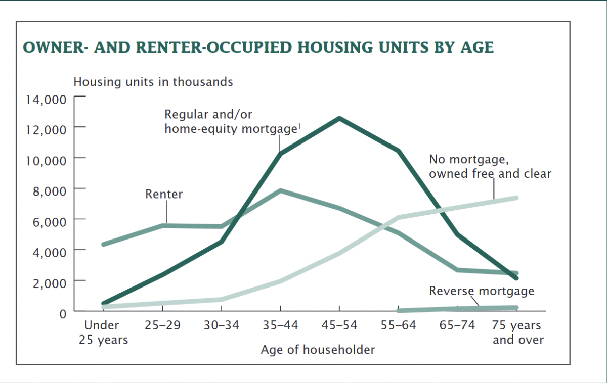
Activity
Run code to show the graph render
Hopefully, you got a similar graph to the one above. If you’re having any issues let your instructor know!
Households with young children and no internet connection at home
Let’s get more insights from our data! One question we can ask is `What is the proportion of households with children younger than 15 do not have an internet connection at home in each state?’
To answer this question, we will need to use the data both from the person and the housing datasets. The person dataset has the age of all the respondants to the survey, while the housing dataset has the information about whether the house has an internet connection. The two datasets can be joined on the SERIALNO column.
First, we’ll start by finding the households that have children 15 years old or younger (with_kids).
person = ibis.read_parquet("partitioned_people/RT=P/*/*.parquet",hive_partitioning=True)

with_kids = (
    person
    .filter(_.AGEP <= 15)
    .select("SERIALNO", "ST")
    .distinct()
)
Now that we have identified the households with children who are less than 15 years old, let’s estimate how many of them do not have an internet connection. To this end, we are going to join the with_kids table we just created with the household table using the SERIALNO field. We can then filter the dataset to only keep the households with no internet access represented with “3” in the ACCESSINET column. We’ll also use mutate to turn the ST column into a string column so we can join this table with another one in just a bit!
no_internet_households_by_state = (
    household
    .join(with_kids, with_kids.SERIALNO == _.SERIALNO)
    .filter((_.ACCESSINET.notnull()) & (_.ACCESSINET == 3))
    .drop('ST_y')
    .relabel({"ST_x": "ST"})
    .group_by('ST')
    .count()
    .relabel({"count": "household_no_internet"})
)

no_internet_households_by_state = no_internet_households_by_state.mutate(ST = _.ST.cast('string'))

no_internet_households_by_state.head()
Then, we will tally up the total number of households with children under 15 for each state:
total_households_by_state = (
    with_kids
    .group_by('ST')
    .count()
    .relabel({"count": "total_households"})
)
We can now return the proportion of the houses with children that do not have internet access. We will also join the pums_state table which contains the names of each state so we can more easily interpret the results.
states = ibis.read_csv("pums_states.csv").mutate(pums_code = _.pums_code.cast('string'))
res = (
    total_households_by_state
    .join(no_internet_households_by_state, no_internet_households_by_state.ST == total_households_by_state.ST)
    .mutate(
        prop = (_.household_no_internet/_.total_households) * 100
    )
    .join(states, states.pums_code == _.ST)
)

res.order_by(ibis.desc(_.prop))
Activity
Run this code and show the resulting table.
Great work! For the last part of this tutorial we’ll switch to a remote database and answer a few more questions but using another backend.